Superficially, a valuation methodology exists to help an investor estimate, within a reasonable range, how much something is worth. Investing, however, is not merely an intellectual exercise. The fundamental problem that an investor faces is that, while it is absolutely essential to invest in order to grow one’s wealth, the nature of risk is such that investing is more likely to destroy wealth than create it. This tendency toward wealth destruction is what Daniel Bernoulli called, “nature’s admonishment to avoid the dice”. The true purpose of a valuation methodology is to guide the investor toward those investment opportunities that offer returns greater than those earned by the market, while not exposing one to the risks of wealth destruction. The following valuation methodology, grounded upon a series of accounting adjustments I make, represents my process for estimating the intrinsic value of a business, or what I, following New Constructs, call its “economic book value”.

Principles and Definitions

An investor is, before anything, a reader in search of truth, a probabilistic truth scattered across the pages of periodic reports. Benjamin Graham and David Dodd summed up the investor’s mission thus:

In all of these instances he appears to be concerned with the intrinsic value of the security and more particularly with the discovery of discrepancies between the intrinsic value and the market price.

Security Analysis, by Benjamin Graham and David Dodd

The question remains, what is intrinsic value? Perhaps the best definition of intrinsic value is one proffered by Jesse Livermore of the perceptive Philosophical Economics blog, where he says, “The ‘intrinsic value’ of a security is the maximum price that an investor would be willing to pay to own the security if he could not ever sell it”. In other words, it is the maximum economic benefit if a shareholder was forced to hold a stock for the remainder of its life, and so, mathematically, it is equivalent to the present value of the cash that can be taken out of a business during the remainder of its life. It is noteworthy that John Burr Williams opened his ground-breaking, The Theory of Investment Value, with the words, “Separate and distinct things not to be confused, as every thoughtful investor knows, are real worth and market price…”, and went on to show that the “real worth” of a business could be determined by an “evaluation by the rule of present worth”. Consequently, a business’ intrinsic value is equal to the present value of its future net cash flows. 

Since 1890, when Alfred Marshall published his Principles of Economics, we have known that the value, or economic benefit that arises from owning a business, is created when that business grows its revenue, and earns a return on invested capital (ROIC) in excess of the opportunity cost, or what standard financial theory now calls the “weighted average cost of capital” (WACC). This is equivalent to the following value driver formula:

Value = [NOPAT(1-g/ROIC)]/(WACC – g)

Here, NOPAT refers to net operating profit after taxes, or the profits that a business’ core operations earn after cash operating taxes have been paid; g refers to growth; ROIC to NOPAT/Invested Capital, where invested capital refers to the cumulative investments into a business; and WACC refers to the economic benefit that could be gained from investing in a similarly risky investment opportunity. 

In practice, one does not use the aforementioned value driver formula given its assumption of constant growth ROIC for the remainder of a security’s life, but it is useful for showing how the value drivers relate. For a single period, value creation can be measured using economic profit, which is ROIC in excess of WACC, scaled by invested capital:

Economic Profit = Invested Capital x (ROIC – WACC)

Discounting a company’s future economic profits and adding that to its starting invested capital, provides one with an estimate of value:

Value = Starting Invested Capital + PV(Projected Economic Profit)

This approach is mathematically equivalent to the discounted cash flow (DCF) valuation. 

Value can also be estimated using the cash-flow perpetuity formula, which assumes a constant growth rate, such that,

Value = FCF/(WACC – g)

Here, FCF refers to free cash flow, that is, the cash flows generated by a business’ core operations, after paying for incremental investments, or increase in invested capital.

FCF = NOPAT – Incremental Investment

The value principle comes with a corollary, what Richard Brealey, Stewart Myers, and Franklin Allen, in their textbook, Principles of Corporate Finance, refer to as the law of conservation of value: any activity that does not increase cash flows does not create value. One early application of this principle is the work of Merton Miller and Franco Modigliani, who showed that a business’ capital structure is irrelevant to its value, unless that capital structure changes the business’ cash flows. 

Since 1890, we have also known that, over the long run, returns are driven down toward WACC, as a result of a gravitational pull of competition. The period in which a business can earn an economic profit is referred to as the “competitive advantage period”, or “growth appreciation period”. That period’s duration is highly dependent on the ferocity of competition within an industry. In highly competitive industries, value creation is fleeting, and in oligopolistic and monopolistic market structures, value creation is enduring. In Edward Chancellor’s examination of Marathon Asset Management’s capital cycle framework, Capital Returns, he explains the resulting ebbs and flows of capital thus, 

Typically, capital is attracted into high-return businesses and leaves when returns fall below WACC. This process is not static, but cyclical – there is constant flux. The inflow of capital leads to new investment, which over time increases capacity in the sector and eventually pushes down returns. Conversely, when returns are low, capital exits and capacity is reduced; over time, then, profitability recovers. From the perspective of the wider economy, this cycle resembles Schumpeter’s process of “creative destruction” – as the function of the bust, which follows the boom, is to clear away the misallocation of capital that has occurred during the upswing.

This insight by Marathon has been given the imprimatur of academic backing, by way of the asset growth effect. In their paper, “Asset Growth and the Cross-Section of Stock Returns,” economists, Michael Cooper, Huseyin Gulen, and Michael Schill, found that a business’ asset growth is more predictive of its future abnormal returns than traditional value, size and momentum. Returning to the key value driver formula, it can be restated to reflect the corrosive impact of competition. The convergence formula reflects that return on net new investment will converge over time on the WACC, as a business’ competitive advantages are ground down by competition:

Continuing Value = NOPAT/WACC

Here, while a firm may grow, that growth does not result in any value creation whatsoever, as the return on new investment capital (RONIC) equals the opportunity cost. This leads to my measure of intrinsic value, which New Constructs refers to as “economic book value” and which has also been referred to as “pre-strategy value” because it is the perpetuity value of the business before management crafts a strategy to enhance that value:

Economic Book Value = (NOPAT/WACC) – Adjusted total debt (including off-balance sheet debt)  + Excess cash  + Unconsolidated Subsidiary Assets  + Net Assets from Discontinued operations  – Value of Outstanding Employee stock option liabilities  – Under (Over) funded Pensions  – Preferred stock  – Minority interests  + Net deferred compensation assets  + Net deferred tax assets

In order to do all this, the investor must make a series of accounting adjustments that uncover the true economics of a business.

Step 1: Turn Accounting Statements Into Economic Statements

Annual reports are not merely long, and complex, with often abstruse language that seems calculated to befuddle the reader, they are also structured in ways that unintentionally disguise operating performance. To start with, financial statements are not designed to be particularly helpful for an investor seeking to understand the operating performance and value of a business. This is because they mix together core and ancillary business activities and transitory shocks. Income statements commingle operating income with interest expense and other non-core, non-recurring items; balance sheets mush together operating assets, non-operating assets and sources of financing; and cash flow statements blend operating cash flow with investing and financing cash flow. A trivial example from Meta Platform’s income statement from its 2023 10-K will serve as an example of this unhelpful structure:

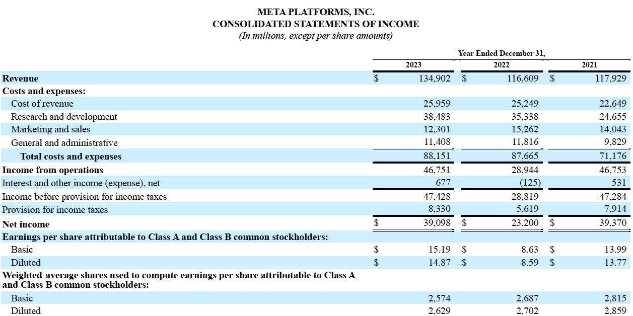
“Interest and other income (expense), net”, are very obviously not part of Meta’s core business activities. This is, as I suggested, is a fairly trivial example, and “income from operations” is a deeply flawed attempt at estimating pre-tax core earnings. An added difficulty is that the elements we need to determine the operating performance of a business are not simply on the face of the financial statement, but they are sprinkled across the annual report, in the MD&A, the footnotes and notes. Moreover, managers are given enormous discretion in classifying items and how they can present disclosures. Further complications are that judgement must be exercised to determine a disclosure’s impact on operating performance and to place each disclosure in the proper economic category. 

Therefore, in order to analyse the operating performance of a business, a rather mundane and yet very important task must be undertaken: the operating, non-operating and sources of financing items of each financial statement must be properly classified, not only on the face of these financial statements, but in the MD&A, the footnotes and notes.

In addition, the auditor’s report is sometimes a source of information about the quality of a firm’s earnings. For instance, in its 2023 annual report, Meta’s auditors, Ernst & Young (EY), pointed to the difficulty in estimating loss contingencies, and “more-likely-than-not to be sustained” federal tax liabilities, interest and penalties sought by the Internal Revenue Service (IRS), and measuring qualifying tax benefits. Such matters usually demand of the reader an analysis of whether existing policies are conservative, and to note any changes in policy and their impact on earnings.

1.1 Create a NOPAT Statement

In their wonderful paper, “Core Earnings: New data and Evidence”, researchers Ethan Rouen, Eric C. So, and Charles C.Y. Wang, present an accurate, rigorous, replicable, and transparent way to estimate core earnings. Their paper is based on an analysis of the remarkable work by financial research firm, New Constructs, who use artificial intelligence and human analysts, to analyse thousands of 10-Ks, and classifies all earnings related quantitative disclosures into their appropriate economic category. At the time the paper was published, New Constructs analysed 60,000 10-Ks, between 1998 and 2017. One of the great achievements of this remarkable paper is that it presents an accurate, rigorous, replicable, and transparent approach to estimating core earnings, while also showing that there is enormous alpha to be gained from having an accurate measure of core earnings. It is that methodology that I use. 

In order to get a sense of the recurring and repeatable profitability of the core business, I calculate its NOPAT. NOPAT excludes income from ancillary business activities and transitory shocks, is independent of a company’s capital structure, and is available not just to shareholders, as with GAAP net income, but to all capital providers. NOPAT must be defined in a way that is consistent with one’s definition of invested capital, so that NOPAT is entirely earned from invested capital. 

This approach uses the same economic categories detailed in New Constructs’ work and Rouen, So and Wang’s paper, with input from that great textbook, Valuation, by Tim Koller et al. A great deal of judgement is involved in placing all the quantitative items into the correct economic adjustment category, as well as the patience to go through an entire annual report, to find both hidden and reported items. By “hidden” is meant those items that are off the face of the income statement, either because they are located in the MD&A or footnotes, or commingled within a reported item; whereas, by “reported” is meant those items that are on the face of the income statement. I calculate NOPAT from both an operating and financing perspective, which are mathematically equivalent, but for the sake of simplicity, below I will only present a detailed reconciliation of Meta’s 2022 GAAP net income with NOPAT, which shows the various adjustments that I make in order to calculate NOPAT, and which are added back to the firm’s GAAP net income.

Adjustments to convert reported GAAP income to NOPAT: 

1. Remove asset write-downs hidden in operating expenses 
2. Remove non-operating expenses hidden in operating earnings 
3. Remove non-operating income hidden in operating earnings 
4. Add back change in reserves 
5. Remove income and loss from discontinued operations (except for REITs) 
6. Add back implied interest for the present value of operating, variable and not-yet commenced leases
7. Add back foreign currency exchange losses and gains
8. Adjust for pension plan costs
9. Adjust for non-operating tax expenses
10. Historical Adjustments: Add back goodwill amortisation and include employee stock option expense prior to accounting changes 
11. Remove reported non-operating items

An example of this is shown below, where I have estimated Meta’s NOPAT for the period 2011 to the last twelve months ending 1Q 2024:

1.2 Create an Invested Capital Statement

Invested capital is the accumulation of investments that have been made into a business’ core operations, in order to earn NOPAT. As with NOPAT, I calculate invested capital from both an operating and financing perspective, but for the sake of simplicity, the adjustments I make will be used to show a detailed reconciliation of Meta Platforms’ total assets to its invested capital. In the abstract, the adjustments to convert reported assets to invested capital are the following: 

1. Add back off-balance sheet reserves 
2. Add back off-balance sheet debt due to operating, variable and not-yet commenced leases 
3. Remove discontinued operations 
4. Remove accumulated Other Comprehensive Income 
5. Add back asset write-downs 
6. Remove deferred compensation assets and liabilities 
7. Remove deferred tax assets and liabilities 
8. Remove under or over funded pensions 
9. Remove excess cash 
10. Prior to 2002: Add back unrecorded and accumulated goodwill 
11. Time-weight acquisitions 
12. Remove non-operating unconsolidated subsidiaries 

Applying this to Meta Platform’s balance sheet gives the following estimate of invested capital for the period 2011 to the LTM:

1.21 Calculate ROIC

With NOPAT and invested capital calculated, calculating ROIC is a trivial affair, simply a matter of dividing NOPAT by average invested capital, which averages invested capital from the beginning and end of the year while also adjusting for the impact of acquisitions during the year. ROIC uncovers the true economics of the company, matching cash returns from cash cumulative investments.

1.22 Calculate Free Cash Flow (FCF) and FCF Yield

FCF, the amount of cash available for distribution to all investors, is the dividend that a company could pay and reflects the profitability of the business. Having already given the formula for FCF in the "Principles and Definitions" section, below is a demonstration of what such a calculation looks like:

FCF Yields are assigned a risk/reward rating using the following classification:

Step 2: Calculate WACC

Next, I calculate the weighted average cost of capital (WACC). WACC is composed to two primary elements: the cost of equity and the cost of debt. I calculate the cost of equity using the capital asset pricing model (CAPM), with beta, its weakest and most controversial component, calculated to express the risk of the stock’s excess returns being lower than that of the market’s in a down market. This is known as D-CAPM. I normalize beta to reduce its impact on my calculations of WACC. For the United States, I use 30-year Treasuries as my risk-free rate. The cost of debt is calculated with the 30-year Treasury bond rate as the risk-free rate added to a spread based on that company’s credit rating, to get the marginal cost of debt. Market values are used, when available, to weight the costs of equity and debt, although, generally, debt values are book values and equity values are market values. 

Step 3: Calculate Economic Profit

Economic profit, as already defined above, is "ROIC in excess of WACC, scaled by invested capital":

Economic Profit = Invested Capital x (ROIC - WACC)

There is a strong correlation between economic profits and market valuation, with a regression by New Constructs of the S&P 500 component companies economic profit and market valuations giving an R² of 0.66854, meaning that 66.854% of market values are explained by economic profits. New Constructs further explained that, "Note that the above regression analysis is based on the 489 companies in the S&P 500 that we cover except for Lorillard (LO). Because of its super high ROIC, including LO in the regression drives the r-squared up to 94%."

The goal of a rationally run business is to create value, which means earning as much economic profit as is possible. It is not surprising that markets reward businesses who achieve this goal. The difficulty is in having the expertise and diligence to make the accounting adjustments necessary to know what a business' true profitability is.

Step 4: Estimate Economic Book Value

Information from the first step will be brought to bear in this stage, to arrive at an estimate of intrinsic value, using economic book value as a measure of the maximum economic benefit that can be derived, based upon proven results, rather than on any attempts at forecasting how management can or will enhance value. The adjustments for economic book value, and indeed, for my discounted cash flow model, enterprise value calculations, are the following:

1. Employee stock option liabilities 
2. Preferred stock 
3. Non-controlling interests 
4. Adjusted total debt (including off-balance sheet debt) 
5. Pension net funded status 
6. Net deferred tax assets or liabilities 
7. Net deferred compensation assets or liabilities 
8. Discontinued operations 
9. Excess cash 
10. Unconsolidated Subsidiaries 

Below follows an estimate of Meta’s economic book value:

The subsequent PEBV ratios can be assessed with the risk/reward system below: